The stacked bar plot has been the poster child (literally on every microbial ecology poster in the past 5 years) of compositional microbial community data visualizations. If you are doing 16S amplicon sequencing and have been given an OTU table with no idea where to go from here, the stacked bar plot may be a good place to start observing trends in your data. Whether or not you move on to some other form of data visualization afterwards is up to you (i.e. Bubble plot).
Load and/or install ggplot2 (for plotting) and reshape2 (for data manipulation) packages. Alternatively, packages like tidyr and dplyr are also great for data manipulation if you prefer
install.packages("ggplot2")
install.packages("reshape2")
library(ggplot2)
library(reshape2)
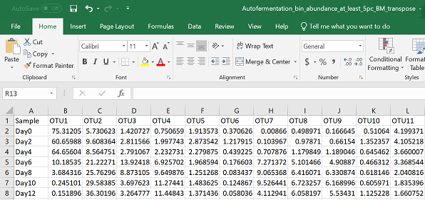
For most analyses in R I find it easiest to upload a csv file that has your species as columns and your samples as rows. Many of the outputs for the 16S pipelines I’ve seen have the order the other way around, so you may have to manipulate and transpose your data to get it in the right orientation (see this tutorial for how to do this in R). I do a lot of my early data manipulations in excel because I find it easiest to 1) get a first glance at the data, and 2) visually observe all the changes I’m making. I can also easily add in extra descriptor columns to define my samples by treatments, or environmental conditions, or any other parameter I could be interested in observing. If you’re a keen coder however, all of these steps are of course possible to do in R. Here are some functions for automated, reproducible data manipulation in R.
Your OTU/species table may have hundreds (or thousands) of OTUs. Obviously, it’s not reasonable or necessary to visualize all these OTUs at once. This is why you may want to select only a few of your most interesting OTUs for this visualization. I tend to choose OTUs for visualization based on criteria like:
- Taxonomy (e.g. Same Phylum)
- Abundance (e.g. At least 1% abundant in one sample)
- Distribution (e.g. Species that change most in abundance)
- Interest (e.g. Any species that are interesting for your story)
E.g.
The following code uses the csv file above as input.
#set your working directory by either setwd()
#or manually in R studio--> Session --> Set Working Directory --> Choose Directory
#upload your data to R - exchange "Your_csv_file.csv" with the name of your csv file
pc = read.csv("Your_csv_file.csv", header = TRUE)
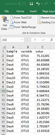
I’ve always found the “wide” and “long” data table formats a difficult concept to explain, especially if you haven’t thought about data in this way before. Briefly, wide data has a column for each variable, whereas long data has one column for all possible variables, and a column for their corresponding values (see figure below). This is important for plotting because ggplot only lets you plot one x variable against one y variable. So if you want to plot multiple species simultaneously in one figure, they need to be in one column (rather than each having its own column).
In the following command I am changing my data structure from a “wide” format to a “long” format. All columns that are not names of OTUs (or species, etc) are placed inside the “id” bracket.
#convert data frame from a "wide" format to a "long" format
pcm = melt(pc, id = c("Sample"))
An example of what the long formatted version of the above data table would like in excel:
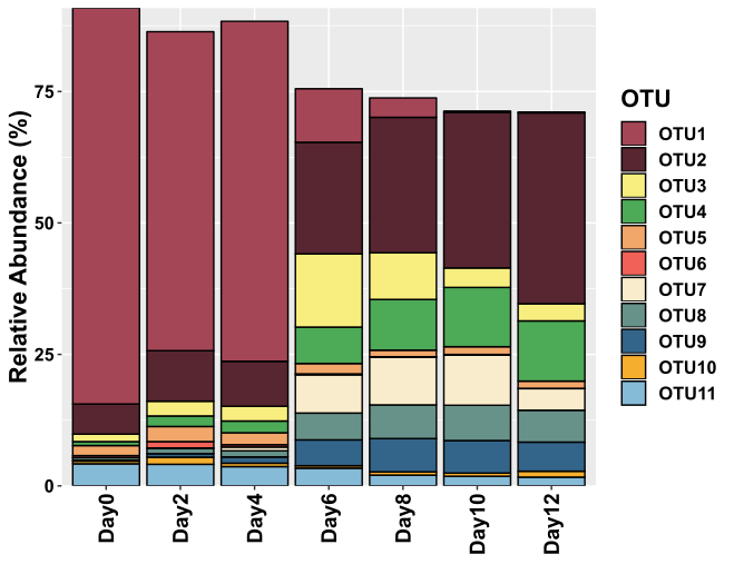
Pick your colours! The following code allows you to define the colours that you will be using in your figure. Stacked bar plots are limited for visualization of data with many variables, because anything over 10 colours on a figure starts to look messy. I have 11 in the figure below, so I’m probably encroaching on messy figure territory here.
P.S. A better way to display abundance data for many (10+) variables/species/OTUs is a Bubble plot.
Picking colours that go nicely together can also be a challenge. I find that using colour scheme generators like this one, can be a good place to start. R understands six digit hex codes, and select colour names that can be found here
The following code creates an object called colours, which contains 11 different colours represented by hex code. I will call upon this object later in my plotting command. Make sure you have at least as many colours as variables.
#define the colours to use in the figure
colours = c( "#A54657",  "#582630", "#F7EE7F", "#4DAA57","#F1A66A","#F26157", "#F9ECCC", "#679289", "#33658A",
"#F6AE2D","#86BBD8")
The following code is useful only if you want to keep the order of your samples the same in your figure as they are in your excel sheet. Otherwise, R will order variables alphabetically.
pcm$Sample <- factor(pcm$Sample,levels=unique(pcm$Sample))
ggplot2 is a fantastic visualization tool once you can get your head around the syntax. You start with code that tells the ggplot command what data frame to use, and then you map your variables to various aesthetics within the “aes” bracket. From there, you can layer on different “geoms” which essentially tell ggplot how you would like to display your data (i.e. bar, point, line).
Try adding each element (the parts before the “+”) one at a time to see how they are changing the plot. There are many different ggplot tutorials out there if you want more information on how to use the package. Here is just one example
#make the plot!
mx = ggplot(pcm, aes(x = Sample, fill = variable, y = value)) +
    geom_bar(stat = "identity", colour = "black") +
    theme(axis.text.x = element_text(angle = 90, size = 14, colour = "black", vjust = 0.5, hjust = 1, face= "bold"),
    axis.title.y = element_text(size = 16, face = "bold"), legend.title = element_text(size = 16, face = "bold"),
    legend.text = element_text(size = 12, face = "bold", colour = "black"),
    axis.text.y = element_text(colour = "black", size = 12, face = "bold")) +
    scale_y_continuous(expand = c(0,0)) +
    labs(x = "", y = "Relative Abundance (%)", fill = "OTU") +
    scale_fill_manual(values = colours)

mx
I’ve started using ggsave almost exclusively for saving my R generated images. It’s awesome because you can save your figures as svg files, and use a program like Inkscape to make the final edits. Because it’s in an svg format, the layers (i.e. text, points, blocks, etc) added from ggplot can all be edited separately, without distorting other parts of the image.
ggsave("Stacked_bar_plot.svg")
Once you have an overview of how your microbiome data looks, you may want to dig deeper to find out the factors influencing microbial distribution through: