Mantel tests are correlation tests that determine the correlation between two matrices (rather than two variables). When using the test for microbial ecology, the matrices are often distance/dissimilarity matrices with corresponding positions (i.e. samples in the same order in both matrices). In order to calculate the correlation, the matrix values of both matrices are ‘unfolded’ into long column vectors, which are then used to determine correlation. Permutations of one matrix are used to determine significance. Learn more about Mantel tests here.
A significant Mantel test will tell you that the distances between samples in one matrix are correlated with the distances between samples in the other matrix. Therefore, as the distance between samples increases with respect to one matrix, the distances between the same samples also increases in the other matrix.
I find this is a difficult concept to explain without defining what the matrices are composed of, so here are some examples:
- Species abundance dissimilarity matrix: created using a distance measure, i.e. Bray-curtis dissimilarity. This is the same type of dissimilarity matrix used when conducting an ANOSIM test or when making an NMDS plot
- Environmental parameter distance matrix: generally created using Euclidean Distance (i.e. temperature differences between samples)
- Geographic distance matrix: the physical distance between sites (i.e. Haversine distance)
With these matrix examples, you could determine if the differences in community composition between samples are correlated, or rather “co-vary”, with the differences in temperature between samples, or the physical distance between samples. These tests can be used to address whether the environment is “selecting” for the microbial community, or if there is a strong distance decay pattern, suggesting dispersal limitation. These are important questions in studies of Microbial Biogeography
To perform a Mantel test in R. First load/install the required packages. The Mantel test function is part of the vegan package, which is also used for anosim tests and nmds plots.
library(vegan)
install.packages("geosphere")
library(geosphere)
If you are interested in using physical distance between samples as a matrix for the Mantel test. The package geosphere contains a function for calculating Haversine distances (distance between two points on a sphere) given latitude and longitude.
Next load in your data with columns as OTUs/variables, and rows as samples.
df = read.csv("Your_OTU_table.csv", header= TRUE)
The data I’m using looks like this:
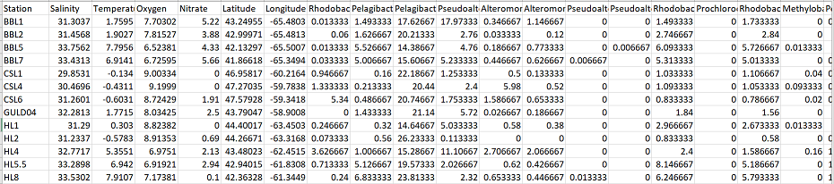
The first column is sample name, the next 4 columns contain environmental parameters for each sample (i.e. Salinity, Temperature, etc). Then, the following 2 columns contain the latitude and longitude for each sample, and the remaining columns contain the 200+ OTU abundances that correspond to each sample.
Now I need to subset my data into smaller data frames/vectors that contain just the information I need to generate the corresponding distance matrices. I will make three subsets: an abundance data frame, a vector with temperature info, and a data frame with the latitude and longitude of my samples. My OTU data starts at column 8. In the code below change the ‘8’ to the column where your OTU data starts. Change the environmental parameter name (‘Temperature’) to whatever it is named in your data.
#abundance data frame
abund = df[,8:ncol(df)]

#environmental vector
temp = df$Temperature

#longitude and latitude
geo = data.frame(df$Longitude, df$Latitude)
Now we have to convert these subsets into distance matrices.
#abundance data frame - bray curtis dissimilarity
dist.abund = vegdist(abund, method = "bray")

#environmental vector - euclidean distance
dist.temp = dist(temp, method = "euclidean")

#geographic data frame - haversine distance
d.geo = distm(geo, fun = distHaversine)
dist.geo = as.dist(d.geo)
Now we can run the mantel command:
#abundance vs environmental
abund_temp = mantel(dist.abund, dist.temp, method = "spearman", permutations = 9999, na.rm = TRUE)
abund_temp

#abundance vs geographic
abund_geo  = mantel(dist.abund, dist.geo, method = "spearman", permutations = 9999, na.rm = TRUE)
abund_geo
The mantel command requires the user to specify certain parameters:
- distance matrices (i.e. dist.abund and dist.temp)
- correlation method. I use Spearman to make the test “non-parametric”. Learn more about correlation methods here
- permutations. Mantel tests determine significance by permuting (randomizing) one matrix X number of times and observing the expected distribution of the statistic. I tend to pick a larger permutation number, but if computing power is low, feel free to decrease
- na.rm. An optional addition to the command that tells R to delete rows in which there are missing values.
The output of these Mantel tests are:
#abundance vs temperature test
> abund_temp

Mantel statistic based on Spearman's rank correlation rho

Call:
mantel(xdis = dist.abund, ydis = dist.temp, method = "spearman", permutations = 9999, na.rm = TRUE)

Mantel statistic r: 0.677
      Significance: 1e-04

Upper quantiles of permutations (null model):
  90%   95% 97.5%   99%
0.148 0.198 0.246 0.290
Permutation: free
Number of permutations: 9999


#abundance vs geography test
> abund_geo

Mantel statistic based on Spearman's rank correlation rho

Call:
mantel(xdis = dist.abund, ydis = dist.geo, method = "spearman", permutations = 9999, na.rm = TRUE)

Mantel statistic r: 0.1379
      Significance: 0.0525

Upper quantiles of permutations (null model):
  90%   95% 97.5%   99%
0.107 0.140 0.170 0.204
Permutation: free
Number of permutations: 9999
From the results, I can see that the temperature distance matrix has a strong relationship with the species Bray-Curtis dissimiliarity matrix (Mantel statistic R: 0.667, p value = 1e-04). In other words, as samples become more dissimilar in terms of temperature, they also become more dissimilar in terms of microbial community composition.
In contrast, the species Bray-Curtis dissimilarity matrix did not have a significant relationship with the geographic separation of the samples (Mantel statistic R: 0.138, p value = 0.052). Therefore, as samples became physically more separated their corresponding microbial communities didn’t necessarily become more dissimilar.
If I was interested in investigating the effect of my environmental variables on my microbial community structure further, I would swap out “Temperature” in the above code, and trade in “Salinity” or “Nitrate”. Alternatively, if I was interested in the total effect of environmental parameters on my microbial community, I could combine all environmental parameters into one distance matrix and test the correlation of this matrix with my abundance data:
#create environmental data frame
#make subset
env = df[,2:5]

#scale data
scale.env = scale(env, center = TRUE, scale = TRUE)

#create distance matrix of scaled data
dist.env = dist(scale.env, method = "euclidean")

#run mantel test
abund_env = mantel(dist.abund, dist.env, method = "spearman", permutations = 9999, na.rm = TRUE)
abund_env
In this case we need to scale the environmental data prior to creating a distance matrix. This is because the environmental variables were all measured using different metrics that are not comparable to each other.
Mantel test output for all environmental parameters:
##Mantel statistic based on Spearman's rank correlation rho

Call:
mantel(xdis = dist.abund, ydis = dist.env, method = "spearman",      permutations = 9999, na.rm = TRUE)

Mantel statistic r: 0.6858
      Significance: 1e-04

Upper quantiles of permutations (null model):
  90%   95% 97.5%   99%
0.151 0.201 0.244 0.292
Permutation: free
Number of permutations: 9999
The results show again that the cumulative environmental factors are strongly correlated with the microbial community (Mantel statistic r: 0.686, p value = 1e-04). Because the microbial community is more strongly correlated with the environmental parameters than the geographic distance, I would draw the conclusion that in this system, the environment is “selecting” for the microbial community, and there is minimal (or comparatively minimal) dispersal limitation occurring.
Stating the statistical values from the Mantel test is a sufficient way to report the results of these tests. I also think that plotting the correlation as a pairwise scatter plot can be an intuitive way to show these rather complex relationships. Check out this tutorial to see how to make scatter plots in R.