When analyzing microbial data, you may want to identify microbial species that are found more often in one treatment group compared to another. There are a number of ways to find these differentially abundant species, all of which use slightly different methods. Generally however, I’ve found that these different methods should all reach similar conclusions. SIMPER , mvabund and Indicator Species Analysis (below) are examples of statistical tests used to find differentially abundant species.
Indicator species are:
“A species whose status provides information on the overall condition of the ecosystem and of other species in that ecosystem. They reflect the quality and changes in environmental conditions as well as aspects of community composition.” - United Nations Environment Programme (1996)
In order to perform indicator species analysis you need an OTU table, or something similar, that contains all the information about your species distributions across your samples. You also need corresponding data that assigns these same samples to groups. The groups you use can be habitat type, treatment, time, etc. I often use the same groups that I use for the ANOSIM statistical test. This way I can check to see which species are most responsible for the differences in microbial community composition between my groups.
There is a specific R package to perform Indicator Species Analysis called indicspecies, developed by the authors of this paper. They also have a thorough tutorial if you want more information. To begin, load and install the indicspecies package. Then load in your data. I find it easiest if your data is in the format of columns as OTUs and rows as samples.
install.packages("indicspecies")
library(indicspecies)
pc = read.csv("Your_OTU_table.csv", header= TRUE)
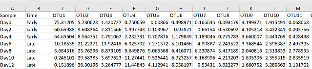
In this case, I have one column called “Time”, that contains the information for grouping my samples into “Early” and “Late” categories. Next I want to create a data frame with all my abundance data, and a vector that contains the information from the “Time” column:
abund = pc[,3:ncol(pc)]
time = pc$Time
Because my abundance data starts in the 3rd column of my original “pc” data frame. I put a “3” in the code above. Change this number to match the column where your abundance data starts. Also change “Time” to whatever you have called your grouping variable.
Next we can run the indicator species command:
inv = multipatt(abund, time, func = "r.g", control = how(nperm=9999))
multipatt is the name of the command from the indicspecies package. The mulitpatt command results in lists of species that are associated with a particular group of samples. If your group has more than 2 categories, multipatt will also identify species that are statistically more abundant in combinations of categories.
The parameters for multipatt are as follows:
- the community abundance matrix:"abund"
- the vector that contains your sample grouping information: "time"
- the function that multipatt is using to identify indicator species: func = "r.g"
- the number of permutations used in the statistical test: control = how(nperm=9999)
The statistic value for the “r.g” function in the indicator species test is a “point biserial correlation coefficient”, which measures the correlation betweeen two binary vectors (learn more about the indicator species method here). Depending on your computing power, 9999 permutations might be too many. Feel free to decrease this number.
To view the results:
summary(inv)
The summary function will only return the statistically significant species ( p < 0.05). If you are interested in all your species, add alpha = 1 to your command. The output of summary looks like:
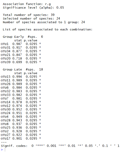
From this output, I can see that the significance level being reported is 0.05, and that the function “r.g” was used. There were 39 species tested in total. 24 of these were significantly associated with one group.
The first list contains the species found significantly more often in the “Early” grouping. The #sps 6 shows that 6 species were identified as indicators for this group. The first column contains species names, the next column contains the stat value (higher means the OTU is more strongly associated). The p.value column contains the statistical p values for the species association (lower means stronger significance). The final column shows the significance level, which is explained by the Signif. codes at the bottom of the output.
Below this first list are the species associated with the other group, “Late”. There are 18 species significantly associated with this group. In both cases, the species are listed in order with strongest association at the top.
I use these results to help me get an initial overview of the species that might be more interesting to investigate. To display these results visually, I often use a boxplot to show the differences in distribution of these identified, statistically significant species between my groupings.