Error bars with ggplot2

Error bars show the range of variability associated with a value around the mean of that value. This variability can be representative of natural variations, uncertainty, or error, and can be caluculated from a number of measures for variation including standard deviation, standard error, range, and confidence intervals. Incorporating error bars into plots (like bar plots) in R is actually not as straightforward as you might expect, so I’ve put together this tutorial based on my trials and tribulations with this process.

There are two general ways to approach error bars in R:

1. Come with your averages and variability already calculated and included in your data frame
2. Calculate your averages and variability based on your data in R

Averages and variability already calculated

I’ll start with method 1 which assumes you have already calculated averages and variability for your samples.

One Variable

Here is an example of the layout for your data with variables/categories as rows, and averages and standard deviation (calculated already in excel), as columns. In the first example, I’m going to use simple data where I only have one variable.

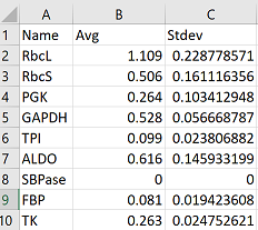
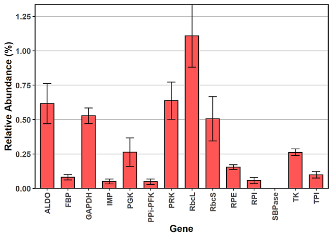
Here the data is already in the correct format so we can plot it right away with ggplot2. In the code below, you will need to change “Name” to whatever you’ve named your category column.

xx = ggplot(df, aes(x = Name, y = Avg, ymin = Avg-Stdev, ymax = Avg+Stdev)) + 
	geom_bar(colour = "black", stat = "identity", width = 0.65, fill = "#ff5555") + 
	geom_errorbar(colour = "black", stat = "identity", width = 0.4) + 
	theme(axis.text.x = element_text(size = 9.5, face = "bold", angle = 90,hjust = 1, vjust = 0.5), 
	axis.title = element_text(size = 12, face = "bold"), axis.text.y = element_text(size = 10, face = "bold"), 
	panel.background = element_blank(), panel.border = element_rect(size = 1, fill = NA, colour = "black"), 
	panel.grid.major.x = element_blank(), panel.grid.major.y = element_line(colour = "grey80")) + 
	labs(x = "Gene", y = "Relative Abundance (%)") + 
	scale_y_continuous(expand = c(0,0))
	
xx

#save your figure
ggsave("your_figure.svg")

In order to include error bars with ggplot2 plots, you need to add the layer geom_errorbar and specify the ymin and ymax in your aesthethics, either for the plot, or within geom_errorbar. Here ymax and ymin refer to the top and bottom of the error bars, and in order to calculate these values, you need to add and subtract your standard deviation from your average.

### Example from the previous code: 
### ymin = Avg - Stdev
### ymax = Avg + Stdev

Multiple Variables

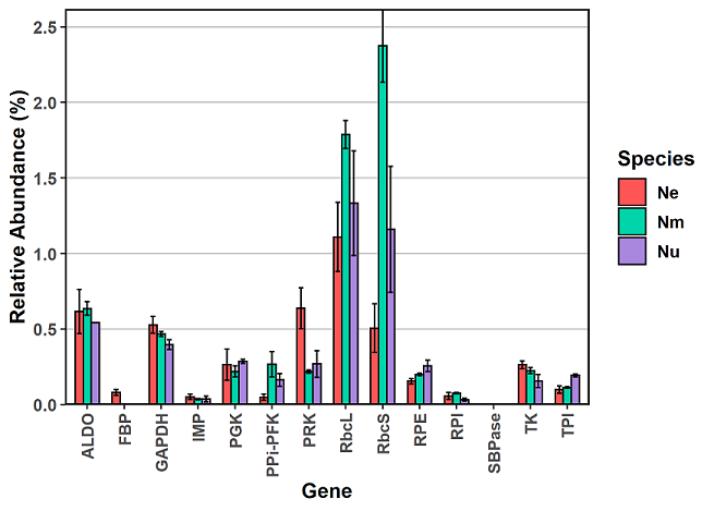
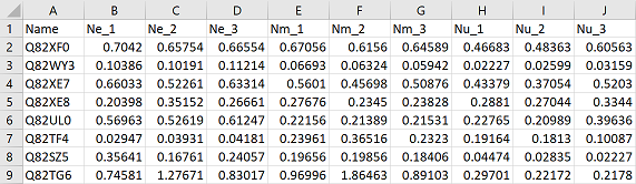
Now what if you have more than one variable? In this example I have three species: Ne, Nm, Nu. The first column lists the gene name, columns 2-4 show average expression per species. Columns 5-7 show standard deviation of the replicates for each species.

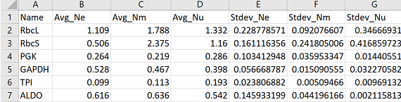
It’s easier for the next steps if you name your columns in a format that specifies in a repeatable manner which columns are averages and which are standard deviations. For example, in this data, the prefixes “Avg_”, and “Stdev_” are added to specify that the values are averages and standard deviations respectively.

Next we load our data into R, and set up the required packages. The library tidyverse contains all Hadley Wickham’s tidy packages, including ggplot2 for data visualization, and dplyr for data manipulation.

library(tidyverse)

df = read.csv("your_data.csv", header = TRUE)

From here we need to do a bit of manipulation to get the data in the correct format for plotting. This format is called “long” format, and I talk about it more in other tutorials

df2 = df %>% 
    gather(desc, value, -Name) %>% 
    separate(desc, c("Stat", "Var")) %>% 
    spread(Stat, value)
    
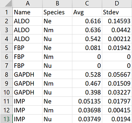
head(df2)

This code rearranges your data so that you end up with a column for your initial categories (in my case genes), a column for variable (in my case species), a column for your average, and a column for standard deviation. You will need to change “Name” to whatever you’ve named your category column. The command separate separates the names of your original columns based on a separator character, in this case an underscore. This is why it is helpful to name your original columns with prefixes or suffixes that can be easily separated. Try running each line of code on its own (before the pipe, %>%) to determine what is occurring at each step.

Now we can plot with ggplot2. This code is basically the same as the code for one variable. However, it now includes extra information for including a legend and for defining fill colours. Within the geom_bar layer, the “width” parameter makes the bars skinnier, and the “position” parameter in geom_errorbar helps to align the errorbars with their respective bar. Otherwise, they all get annoyingly plotted on top of each other.

xx = ggplot(df2, aes(x = Name, y = Avg, ymin = Avg-Stdev, ymax = Avg+Stdev, fill = Species)) + 
	geom_bar(colour = "black", stat = "identity", position = "dodge", width = 0.65) +      	
	geom_errorbar(colour = "black", stat = "identity", position = position_dodge(0.65), width = 0.4) + 
	theme(axis.text.x = element_text(size = 9.5, face = "bold", angle = 90,hjust = 1, vjust = 0.5), 
	axis.title = element_text(size = 12, face = "bold"), axis.text.y = element_text(size = 10, face = "bold"), 
	legend.text = element_text(size = 10, face= "bold"), panel.background = element_blank(), 
	panel.border = element_rect(size = 1, fill = NA, colour = "black"), 
	panel.grid.major.x = element_blank(), panel.grid.major.y = element_line(colour = "grey80"), 
	legend.title = element_text(size = 12, face = "bold")) + 
	labs(x = "Gene", y = "Relative Abundance (%)", fill = "Species") + 
	scale_y_continuous(expand = c(0,0)) + 
	scale_fill_manual(values = c( "#ff5555", "#00d4aa", "#aa87de"))

xx

#save your figure
ggsave("your_image.svg")

Calculate averages and variability in R

Okay so here is a workflow if you’ve decided to import raw data without averages and variability already calculated. The following code works if your data is in the format of one column containing variables/categories (“Name”), and the remaining columns as numeric values corresponding to sample replicates. Again, it helps if you name your sample columns in an intuitive way. In my data, I have the species abbreviation first, followed by an underscore and the replicate number: i.e. “Ne_1”. This will make it easier to separate the species information from the replicate information later on.

First load in your data and libraries

library(tidyverse)
df = read.csv("your_data_frame.csv", header = TRUE)

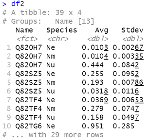
Next we need to summarize our data so that we calculate the average and standard deviation for each variable for each category. We will end up with a data frame that has a column for category, a column for species, and then a column for the corresponding average, and a column for the corresponding standard deviation. sd is the R command for standard deviation. If you would like to use a different metric of variability, change the sd command in the code accordingly.

df2 = df %>% 
    gather(sample, value, -Name) %>%
    separate(sample, c("Species", "replicate")) %>%
    group_by(Name, Species) %>%
    summarize(Avg = mean(value), Stdev = sd(value))

head(df2)

This code uses a series of data manipulation commands from the dplyr package within the tidyverse suite of packages. Try running each line of code separately (before the pipe symbol, %>%) to get a better idea of what each command is doing. If your data was in a slightly different format to begin with, you may need to tweak some of the code. *From here you can run the exact same *ggplot2 command that generated the plot above. Good luck!